Real-time Speaker Diarization

Speaker diarization answers the fundamental question: "who spoke when?" In real-time applications—from live transcription to virtual meetings—identifying speakers as they talk presents unique challenges that batch processing doesn't face. This article explores a practical approach to real-time speaker diarization using K-means clustering, agglomerative clustering, and neural speaker embeddings.

The Challenge of Real-time Diarization

Traditional speaker diarization systems process complete audio files, allowing multiple passes over the data. Real-time systems must:

• Process incrementally: Make decisions with incomplete information
• Maintain low latency: Deliver results within acceptable delay thresholds
• Handle dynamic speakers: Adapt as new speakers join the conversation
• Update continuously: Refine speaker assignments as more data arrives

Our approach addresses these challenges by combining fast initial clustering with refinement as context accumulates.

The Algorithm Approach

The diarization pipeline follows these steps:

1. Generate speaker embeddings from each transcribed sentence
2. Use K-means to detect whether we have one or multiple speakers
3. Apply Agglomerative Clustering for multi-speaker scenarios
4. Calculate silhouette scores to determine optimal speaker count
5. Assign sentences to speakers by cluster membership

This hybrid approach leverages K-means for speed and agglomerative clustering for accuracy when speaker count is unknown.

Speaker Embeddings

Speaker embeddings are dense vector representations that capture the unique characteristics of a voice, think of them as voice fingerprints. These high-dimensional vectors encode pitch, timbre, speaking style, and other acoustic features that distinguish one speaker from another.

Understanding Multi-Scale Embeddings

Modern speaker embedding models employ a multi-scale approach to capture voice characteristics at different temporal resolutions. This technique significantly improves speaker discrimination by analyzing speech patterns across multiple window sizes.

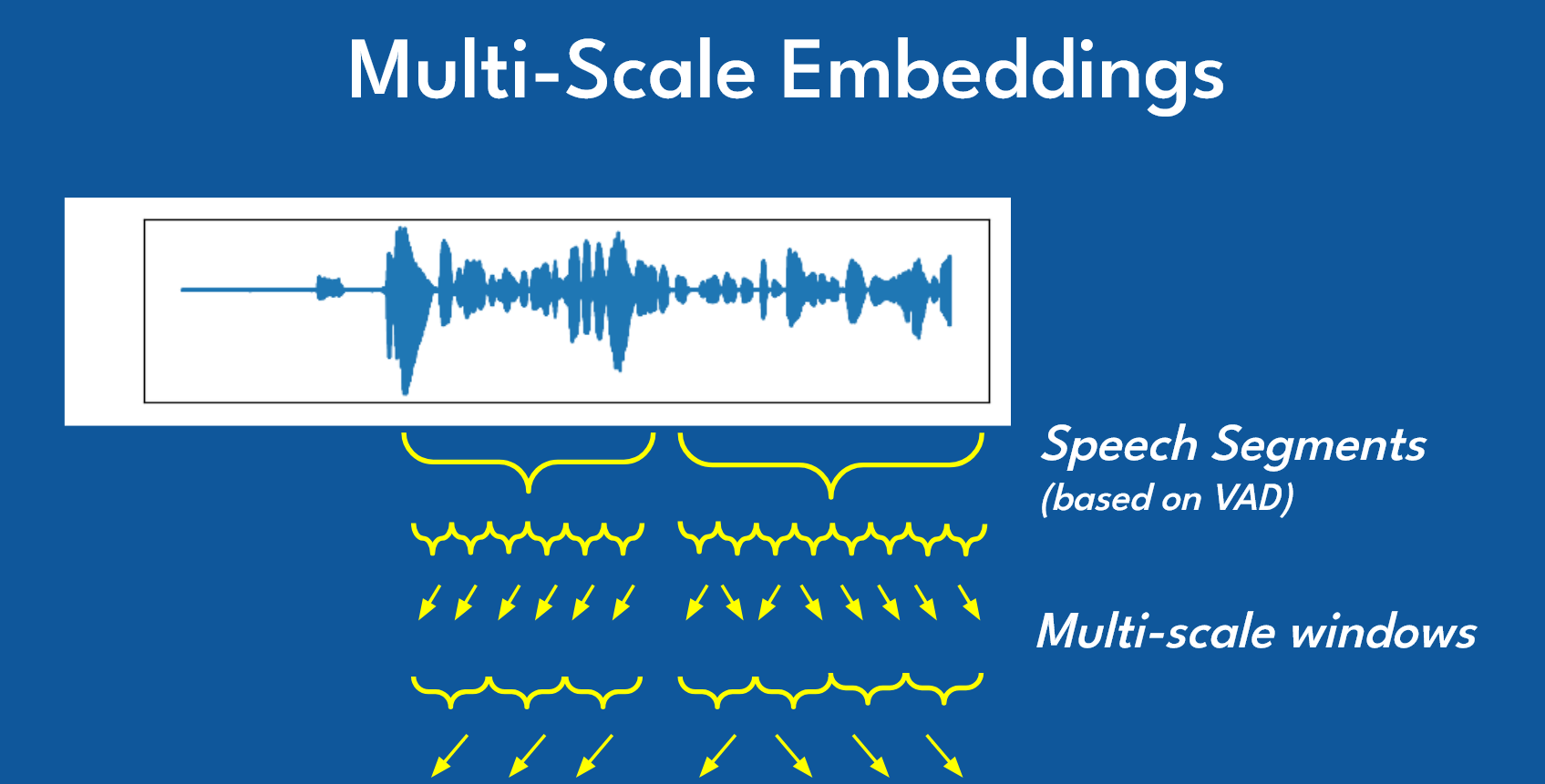
The diagram above illustrates the multi-scale embedding extraction process:

1. Speech Segmentation: Voice Activity Detection (VAD) first identifies speech segments from the continuous audio waveform, filtering out silence and non-speech noise.

2. Multi-Scale Windows: Each speech segment is then analyzed using windows of varying lengths. Shorter windows capture rapid acoustic transitions (like phoneme boundaries), while longer windows encode prosodic features (like intonation patterns and speaking rhythm).

3. Hierarchical Feature Extraction: These windows are processed through the embedding model at multiple scales, creating a rich representation that captures both fine-grained spectral details and broader temporal characteristics.

4. Embedding Aggregation: The multi-scale features are combined into a single fixed-dimensional vector that serves as a unique "voice fingerprint" for speaker identification.

This multi-scale strategy is why modern embedding models like Resemblyzer, Pyannote, and Coqui TTS achieve high accuracy in distinguishing between speakers, even those with similar vocal characteristics.

Option A: Coqui TTS

Coqui TTS, while primarily a text-to-speech model, provides excellent speaker embeddings through its conditioning latent extraction:

from TTS.tts.models import setup_model as setup_tts_model
from TTS.config import load_config
import torch
import os

# Load the TTS model
device = torch.device("cuda" if torch.cuda.is_available() else "cpu")
local_models_path = os.environ.get("COQUI_MODEL_PATH")
checkpoint = os.path.join(local_models_path, "v2.0.2")
config = load_config(os.path.join(checkpoint, "config.json"))

tts = setup_tts_model(config)
tts.load_checkpoint(
    config,
    checkpoint_dir=checkpoint,
    checkpoint_path=None,
    vocab_path=None,
    eval=True,
    use_deepspeed=False,
)
tts.to(device)

# Extract speaker embedding from audio
def get_speaker_embedding(audio_path):
    _, speaker_embedding = tts.get_conditioning_latents(
        audio_path=audio_path,
        gpt_cond_len=30,
        max_ref_length=60
    )
    # Flatten to 1D numpy array
    return speaker_embedding.view(-1).cpu().detach().numpy()

Option B: Resemblyzer

Resemblyzer is a lightweight library specifically designed for speaker verification using d-vectors:

from resemblyzer import VoiceEncoder, preprocess_wav
from pathlib import Path
import numpy as np

# Load the encoder (downloads model on first use)
encoder = VoiceEncoder()

def get_speaker_embedding_resemblyzer(audio_path):
    # Preprocess and encode
    wav = preprocess_wav(Path(audio_path))
    embedding = encoder.embed_utterance(wav)
    return embedding  # 256-dimensional vector

Option C: Pyannote

Pyannote-audio is the industry standard for speaker diarization, offering pre-trained pipelines:

from pyannote.audio import Model, Inference
import torch

# Load pretrained embedding model
model = Model.from_pretrained(
    "pyannote/embedding",
    use_auth_token="YOUR_HF_TOKEN"
)
inference = Inference(model, window="whole")

def get_speaker_embedding_pyannote(audio_path):
    embedding = inference(audio_path)
    return embedding  # 512-dimensional vector

Comparison

Feature	Coqui TTS	Resemblyzer	Pyannote
Embedding Dim	512	256	512
Speed	Medium	Fast	Medium
Accuracy	High	Good	Excellent
GPU Required	Recommended	No	Recommended
Model Size	Large	Small	Medium
Primary Use	TTS + Embeddings	Speaker Verification	Full Diarization

Choose Resemblyzer for lightweight applications, Pyannote for production diarization pipelines, and Coqui TTS if you're already using it for text-to-speech synthesis.

K-Means for Speaker Detection

K-means provides a fast initial check to determine if we're dealing with one speaker or multiple speakers. By clustering embeddings into 2 groups and examining the distances, we can decide whether the audio contains distinct speakers:

from sklearn.cluster import KMeans
from sklearn.preprocessing import StandardScaler
import numpy as np

def determine_speaker_count(embeddings, distance_threshold=17):
    """
    Use K-means to detect single vs multiple speakers.

    Args:
        embeddings: List of speaker embedding vectors
        distance_threshold: Threshold for single speaker detection

    Returns:
        1 if single speaker, otherwise estimated count
    """
    if len(embeddings) <= 1:
        return 1

    # Standardize embeddings
    embeddings_array = np.array(embeddings)
    scaler = StandardScaler()
    embeddings_scaled = scaler.fit_transform(embeddings_array)

    # K-means with k=2
    kmeans = KMeans(n_clusters=2, random_state=0, n_init=10)
    kmeans.fit(embeddings_scaled)

    # Calculate average distance to nearest centroid
    distances = kmeans.transform(embeddings_scaled)
    avg_distance = np.mean(np.min(distances, axis=1))

    # Low distance suggests single speaker
    if avg_distance < distance_threshold:
        print(f"Single speaker detected: distance {avg_distance:.2f} < {distance_threshold}")
        return 1

    return 2  # Multiple speakers detected

The distance threshold is crucial—too low and you'll falsely detect multiple speakers in single-speaker audio; too high and you'll miss speaker changes.

Agglomerative Clustering for Multi-Speaker

When multiple speakers are detected, agglomerative clustering determines the exact count using silhouette scoring:

from sklearn.cluster import AgglomerativeClustering
from sklearn.metrics import silhouette_score

def find_optimal_speakers(embeddings_scaled, max_speakers=10, silhouette_threshold=0.0001):
    """
    Use hierarchical clustering to find optimal speaker count.

    Args:
        embeddings_scaled: Standardized embedding vectors
        max_speakers: Maximum number of speakers to consider
        silhouette_threshold: Minimum improvement to add another speaker

    Returns:
        Tuple of (optimal_count, cluster_labels)
    """
    num_embeddings = len(embeddings_scaled)
    max_clusters = min(max_speakers, num_embeddings)

    silhouette_scores = []

    for n_clusters in range(2, max_clusters + 1):
        hc = AgglomerativeClustering(n_clusters=n_clusters, linkage='ward')
        cluster_labels = hc.fit_predict(embeddings_scaled)

        # Ensure valid clustering
        unique_labels = set(cluster_labels)
        if 1 < len(unique_labels) < len(embeddings_scaled):
            score = silhouette_score(embeddings_scaled, cluster_labels)
            silhouette_scores.append((n_clusters, score))
        else:
            silhouette_scores.append((n_clusters, -1))

    # Find optimal: point before silhouette starts decreasing
    optimal_count = 2
    for i in range(1, len(silhouette_scores)):
        curr_score = silhouette_scores[i][1]
        prev_score = silhouette_scores[i-1][1]

        if curr_score < prev_score + silhouette_threshold:
            optimal_count = silhouette_scores[i-1][0]
            break

    # Get final clustering
    hc = AgglomerativeClustering(n_clusters=optimal_count, linkage='ward')
    final_labels = hc.fit_predict(embeddings_scaled)

    return optimal_count, final_labels

The silhouette score measures how similar samples are to their own cluster compared to other clusters. Higher scores indicate better-defined clusters.

Visualizing Speaker Clusters

When embeddings are projected into 2D space (using techniques like t-SNE or UMAP), we can visualize how the algorithm groups speakers. Each colored point represents a sentence spoken by a particular speaker:

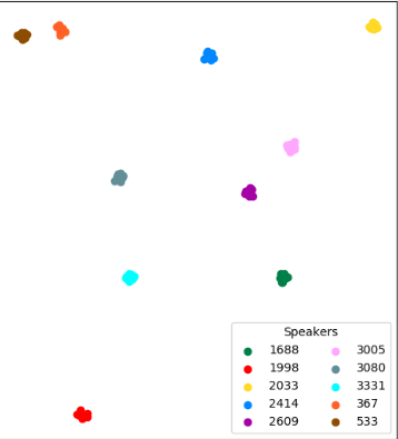
In this visualization, each color represents a different speaker identified by the clustering algorithm. The spatial separation between clusters indicates how distinct the speakers' voices are:

• Well-separated clusters (like the blue cluster at the top and cyan cluster on the left) indicate speakers with very different vocal characteristics
• Closer clusters suggest speakers with more similar voices, which can be more challenging to differentiate
• Cluster tightness reflects consistency—tight clusters indicate consistent voice characteristics across multiple sentences from the same speaker

The speaker IDs (1688, 1998, 2033, etc.) are assigned by the clustering algorithm based on the order speakers are detected. In a real-time system, these assignments update dynamically as new audio arrives and the algorithm refines its understanding of the speaker landscape.

Real-time Implementation

Real-time speaker diarization requires processing audio as it streams in, rather than waiting for complete recordings. The system consists of three concurrent pipelines:

Pipeline Architecture

1. Audio Capture: Continuously read audio chunks from microphone or system audio
2. Speech-to-Text: Transcribe audio in real-time using Whisper
3. Speaker Assignment: Extract embeddings and cluster as new sentences arrive

Core Processing Loop

The key challenge is incremental clustering—every new sentence triggers a complete re-clustering of all accumulated embeddings:

from sklearn.cluster import AgglomerativeClustering, KMeans
from sklearn.preprocessing import StandardScaler
from sklearn.metrics import silhouette_score
import numpy as np
import queue
import wave

class RealtimeSpeakerProcessor:
    """Processes transcribed sentences and assigns speakers in real-time."""

    def __init__(self, embedding_model, sentence_queue):
        self.embedding_model = embedding_model
        self.queue = sentence_queue
        self.full_sentences = []  # (text, embedding) tuples
        self.sentence_speakers = []

        # Tunable thresholds
        self.two_speaker_threshold = 17
        self.silhouette_diff_threshold = 0.0001

    def process_stream(self):
        """Main processing loop - runs continuously."""
        while True:
            text, audio_bytes = self.queue.get()  # Blocking call

            # Extract speaker embedding
            embedding = self.extract_embedding(audio_bytes)
            self.full_sentences.append((text, embedding))

            # Re-cluster ALL embeddings with new data point
            self.update_speaker_assignments()

            # Yield updated results
            yield self.full_sentences, self.sentence_speakers

    def extract_embedding(self, audio_bytes):
        """Convert audio bytes to speaker embedding vector."""
        # Save temporary WAV file
        audio_int16 = np.int16(audio_bytes * 32767)
        temp_file = "temp_audio.wav"

        with wave.open(temp_file, 'w') as wav_file:
            wav_file.setnchannels(1)
            wav_file.setsampwidth(2)
            wav_file.setframerate(16000)
            wav_file.writeframes(audio_int16.tobytes())

        # Extract embedding (example using Coqui TTS)
        _, speaker_embedding = self.embedding_model.get_conditioning_latents(
            audio_path=temp_file,
            gpt_cond_len=30,
            max_ref_length=60
        )
        return speaker_embedding.view(-1).cpu().detach().numpy()

    def update_speaker_assignments(self):
        """Re-cluster all embeddings to assign speakers."""
        embeddings = [emb for _, emb in self.full_sentences]

        if len(embeddings) <= 1:
            self.sentence_speakers = [0] * len(self.full_sentences)
            return

        # Standardize embeddings
        embeddings_array = np.array(embeddings)
        scaler = StandardScaler()
        embeddings_scaled = scaler.fit_transform(embeddings_array)

        # Determine optimal speaker count
        optimal_count = self.determine_speaker_count(embeddings_scaled)

        if optimal_count == 1:
            self.sentence_speakers = [0] * len(self.full_sentences)
        else:
            # Cluster and assign
            hc = AgglomerativeClustering(n_clusters=optimal_count, linkage='ward')
            clusters = hc.fit_predict(embeddings_scaled)

            # Normalize cluster indices
            cluster_mapping = {old: new for new, old in enumerate(set(clusters))}
            self.sentence_speakers = [cluster_mapping[c] for c in clusters]

    def determine_speaker_count(self, embeddings_scaled):
        """Hybrid K-means + silhouette approach."""
        num_embeddings = len(embeddings_scaled)

        if num_embeddings <= 1:
            return 1

        # Step 1: K-means quick check for single vs multiple speakers
        kmeans = KMeans(n_clusters=2, random_state=0, n_init=10)
        kmeans.fit(embeddings_scaled)
        distances = kmeans.transform(embeddings_scaled)
        avg_distance = np.mean(np.min(distances, axis=1))

        if avg_distance < self.two_speaker_threshold:
            return 1  # Single speaker detected

        # Step 2: Silhouette scoring for optimal count
        max_clusters = min(10, num_embeddings)
        silhouette_scores = []

        for n_clusters in range(2, max_clusters + 1):
            hc = AgglomerativeClustering(n_clusters=n_clusters, linkage='ward')
            labels = hc.fit_predict(embeddings_scaled)

            if 1 < len(set(labels)) < len(embeddings_scaled):
                score = silhouette_score(embeddings_scaled, labels)
                silhouette_scores.append(score)
            else:
                silhouette_scores.append(-1)

        # Find elbow point (where improvement drops below threshold)
        optimal = 2
        for i in range(1, len(silhouette_scores)):
            if silhouette_scores[i] < silhouette_scores[i-1] + self.silhouette_diff_threshold:
                optimal = i + 1
                break

        return optimal

Audio Streaming Integration

Connect the processor to a real-time speech-to-text system:

from RealtimeSTT import AudioToTextRecorder
import pyaudio

# Audio configuration
SAMPLE_RATE = 16000
BUFFER_SIZE = 512
FORMAT = pyaudio.paInt16

# Initialize speech-to-text recorder
recorder_config = {
    'model': 'large-v2',
    'language': 'en',
    'silero_sensitivity': 0.4,
    'webrtc_sensitivity': 3,
    'post_speech_silence_duration': 0.4,
    'min_length_of_recording': 0.7,
    'enable_realtime_transcription': True,
    'realtime_model_type': 'distil-small.en',
    'buffer_size': BUFFER_SIZE,
    'sample_rate': SAMPLE_RATE,
}

recorder = AudioToTextRecorder(**recorder_config)

# Setup audio stream
audio = pyaudio.PyAudio()
stream = audio.open(
    format=FORMAT,
    channels=1,
    rate=SAMPLE_RATE,
    input=True,
    frames_per_buffer=BUFFER_SIZE
)

# Feed audio to recorder
def audio_capture_loop():
    while True:
        data = stream.read(BUFFER_SIZE, exception_on_overflow=False)
        recorder.feed_audio(data)

# Process transcriptions
def transcription_loop(sentence_queue):
    def on_sentence_complete(text):
        audio_bytes = recorder.last_transcription_bytes
        sentence_queue.put((text, audio_bytes))

    while True:
        recorder.text(on_sentence_complete)

Key Real-time Considerations

Incremental Clustering: Unlike batch processing, we re-cluster with every new sentence. This allows speaker assignments to evolve as more context accumulates, but introduces computational overhead.

Latency Management: The bottleneck is embedding extraction (~100-300ms per sentence). Use GPU acceleration when available and consider caching embeddings.

Cluster Stability: Early assignments may be unstable with limited data. Consider requiring a minimum number of sentences (e.g., 3-5) before displaying speaker labels.

Memory Management: For long conversations, implement a sliding window or periodically finalize old speaker assignments to prevent unbounded memory growth.

Configuration & Tuning

Key Parameters

Parameter	Default	Description
two_speaker_threshold	17	K-means distance threshold for single speaker detection. Lower = stricter
silhouette_diff_threshold	0.0001	Minimum silhouette improvement to add another speaker
min_length_of_recording	0.7s	Minimum audio length to process
gpt_cond_len	30	Conditioning length for Coqui embeddings
max_ref_length	60	Maximum reference length for embedding extraction

Tuning Tips

1. Single speaker detected when there are two: Lower two_speaker_threshold
2. Two speakers detected when there's one: Raise two_speaker_threshold
3. Too many speakers identified: Raise silhouette_diff_threshold
4. Speakers merged together: Lower silhouette_diff_threshold
5. Poor embedding quality: Increase min_length_of_recording to ensure sufficient audio

Start with default values and adjust based on your specific audio characteristics—background noise, speaker similarity, and microphone quality all affect optimal thresholds.

Conclusion

Real-time speaker diarization combines the speed of K-means clustering with the accuracy of agglomerative clustering to answer "who spoke when" as audio streams in. The hybrid approach—using K-means for quick single/multi-speaker detection and silhouette-scored hierarchical clustering for optimal speaker count—provides a practical balance between latency and accuracy.

Key takeaways:

• Speaker embeddings transform voice characteristics into comparable vectors
• K-means provides fast initial speaker count estimation
• Agglomerative clustering with silhouette scoring determines precise speaker count
• Incremental processing enables real-time applications

Future improvements could include online learning to refine speaker models as more data arrives, speaker identification (matching to known individuals), and handling overlapping speech segments. The modular architecture presented here provides a solid foundation for these enhancements.